Point Calculation
Test Cases for the Procedures Point and PointThruInsertion
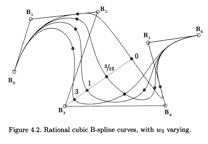
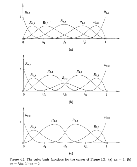
1) The first test of the point calculation algorithms is the case given in The NURBS Book's Figure 4.2-4.3.


The following program tests the point calculation algorithms for curves by reproducing these plots.
program test_curvepoint

use splines
use points

implicit none

integer, parameter :: wp  = selected_real_kind(15,307)
type(curve) :: crv, ratcrv
type(cpt) :: point, a(7)
real(wp) :: U(11)
type(cpt) :: p1(0:4), p2(0:4)

! control points
a(:)%x = [1., 1.25, 3., 1.75, 5., 4., 5.25]; a(:)%y = [1., 2., 2.3, 0., 0., 1.5, 1.8]
! knot vector
U(:) = [0.0_wp,0.0_wp,0.0_wp,0.0_wp,0.25_wp,0.50_wp,0.75_wp,1.0_wp,1.0_wp,1.0_wp,1.0_wp]

! construct a nonrational curve
crv = spl(dim=2, pd=1, p=[3], kXi=U, cp=a )

! plot the curve with control polygon by marking all values of the knot vector over the curve
call crv%plot(plotCP=.true., labelCP=.true., plotElems=.true.,    &
                terminal="png",                     &
                fname="test_F4.2a",                 &
                title="A nonrational cubic B-spline curve, {/symbol w}_{3} = 1")

! plot basis functions
call crv%N(1)%plot(   terminal="png",     &
                        fname="test_F4.3a", &
                        title="Basis functions of the nonrational cubic curve, {/symbol w}_{3} = 1")

! weights w_3=0.3
call a(:)%weighting([1.0_wp, 1.0_wp, 1.0_wp, 0.3_wp, 1.0_wp, 1.0_wp, 1.0_wp])

! construct a rational curve by setting the rational flag to `true`
ratcrv = spl(dim=2, pd=1, p=[3], kXi=U, cp=a ,rat=.true.)

! plot the curve with control polygon by marking all values of the knot vector over the curve
call ratcrv%plot( plotCP=.true., labelCP=.true., plotElems=.true.,    &
                    terminal="png",                     &
                    fname="test_F4.2b",&
                    title="A rational cubic B-spline curve, {/symbol w}_{3} = 0.3")

! plot weighted basis functions
call ratcrv%N(1)%plot(rat=.true., w=a(:)%w,               &
                        terminal="png",                     &
                        fname="test_F4.3b",                 &
                        title="Basis functions of the nonrational cubic curve, {/symbol w}_{3} = 0.3")

! compute the coordinates of the nonrational curve coinciding the knot value "0.5"
call crv%Point(u=0.5_wp,PT=point)

! check values and compare with the plot
print*, point%x, point%y
! =>    2.50000000000000    0.383333325386047

! compute the coordinates of the rational curve coinciding the knot value "0.5"
call ratcrv%Point(u=0.5_wp,PT=point)

! check values from the plot
print*, point%x, point%y
! =>    3.15625000000000    0.718749985098839

! test if curve%point and curve%pointThruInsertion are return the same results
call crv%Point(               [0.0_wp, 0.25_wp, 0.5_wp, 0.75_wp, 1.0_wp], PT=p1(0:4) )
call crv%PointThruInsertion(  [0.0_wp, 0.25_wp, 0.5_wp, 0.75_wp, 1.0_wp], PT=p2(0:4) )
print*, p1==p2
! => T T T T T

call ratcrv%Point(               [0.0_wp, 0.25_wp, 0.5_wp, 0.75_wp, 1.0_wp], PT=p1(0:4) )
call ratcrv%PointThruInsertion(  [0.0_wp, 0.25_wp, 0.5_wp, 0.75_wp, 1.0_wp], PT=p2(0:4) )
print*, p1==p2
! => T T T T T

pause

end program test_curvepoint
The program first reproduces Figure 4.2 with and and Figure 4.3(a)-(b), then computes the coordinates of marked points on the curve to compare different procedures. Besides, the curve%plot command uses the procedure curve%point internally. The resulting plots are as follow,


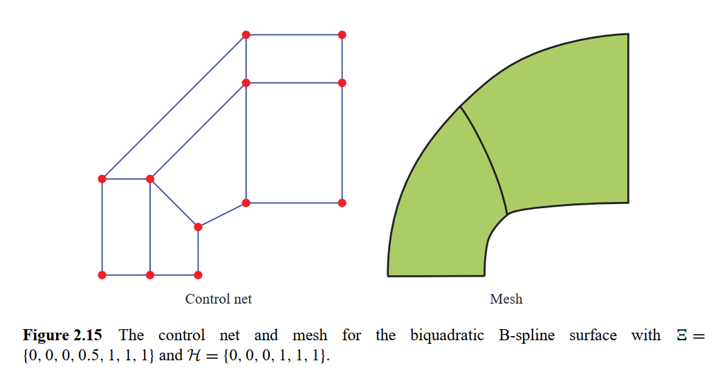
2) The second test of the point calculation algorithms is the case given in Cottrell's IGA book Figure 2.15.

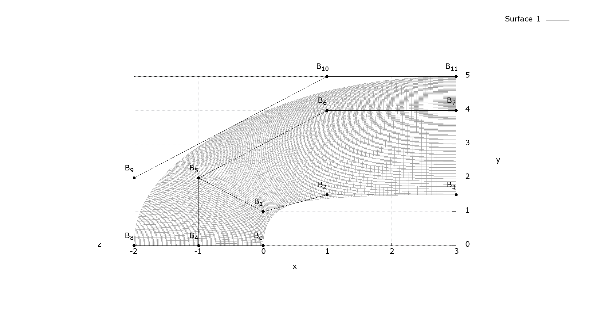
The following program tests the point calculation algorithms for surfaces by reproducing this case.
program test_surfacepoint

use splines
use points

integer, parameter :: wp  = selected_real_kind(15,307)
logical, parameter :: T = 1
logical, parameter :: F = 0
type(surface) :: s
type(cpt) :: point(4)
real(wp) :: U(7),V(6)
type(cpt) :: scp(12)


scp(:)%x = [ 0.0_wp, 0.0_wp, 1.0_wp , 3.0_wp , -1.0_wp, -1.0_wp, 1.0_wp, 3.0_wp, -2.0_wp, -2.0_wp, 1.0_wp, 3.0_wp]
scp(:)%y = [ 0.0_wp, 1.0_wp, 1.50_wp, 1.50_wp,  0.0_wp,  2.0_wp, 4.0_wp, 4.0_wp,  0.0_wp,  2.0_wp, 5.0_wp, 5.0_wp]
!scp(:)%z = [ 0.0_wp, 1.0_wp, 1.0_wp, 0.0_wp,   0.0_wp,  1.0_wp, 1.0_wp, 0.0_wp,  0.0_wp,  1.0_wp, 1.0_wp, 0.0_wp]

U=[0.0_wp, 0.0_wp, 0.0_wp, 0.5_wp, 1.0_wp, 1.0_wp, 1.0_wp]
V=[0.0_wp, 0.0_wp, 0.0_wp, 1.0_wp, 1.0_wp, 1.0_wp]

! dim is set to "three" since surface plots in 2D does not have good looking
s = spl(dim=3, pd=2, p=[2,2], kXi=U, kEta=V, cp=scp)

! plot surface on xy plane (by set view option)
call s%plot(  plotCP=T, labelCP=T,            &
                    terminal='png',                 &
                    fname="testC_F2.15",            &
                    ls="lw 1 lc rgb 'dark-grey'",   &
                    plotOpt=["set view 0,0"])

! calculate the points at the corner of the surface
call s%Point(u=0.0_wp,v=0.0_wp,PT=point(1))
call s%Point(u=1.0_wp,v=0.0_wp,PT=point(2))
call s%Point(u=0.0_wp,v=1.0_wp,PT=point(3))
call s%Point(u=1.0_wp,v=1.0_wp,PT=point(4))

! write the result on the screen
do i=1,4; call point(i)%print(); end do
!=>  0.00000  0.00000  0.00000
!=>  3.00000  1.50000  0.00000
!=> -2.00000  0.00000  0.00000
!=>  3.00000  5.00000  0.00000

pause

end program test_surfacepoint
The plotting algorithm inherently calculates surface points by using the surface%point procedure. Computing the corner points of the surface is also testing the %point routine.
